Five Functional Facts About OSPF
It's funny, in my experience, OSPF is the most widely used interior gateway protocol because it "just works" and it's an IETF standard which means it inter-ops between different vendors and platforms. However, if you really start to look at how OSPF works, you realize it's actually a highly complex protocol. So on the one hand you get a protocol that likely works across your whole environment, regardless of vendor/platform, but on the other you're implementing a lot of complexity in your control plane which may not be intuitive to troubleshoot.
This post isn't a judgement about OSPF or link-state protocols in general. Instead it will detail five functional aspects of OSPF in order to reveal-at least in part-how this protocol works, and indirectly, some of the complexity lying under the hood.
1. OSPF Has Its Own Best Path Decision Process⌗
Ever looked closely at OSPF routes in the show ip route output? You'll notice flags such as O or O IA beside the route.
O     10.1.14.0 255.255.255.0
      [110/21] via 123.1.0.18, 00:00:07, Ethernet0/0
O IA  11.11.11.0 [110/20] via 123.1.0.18, 00:00:07, Ethernet0/0
O IA  123.1.0.20 255.255.255.252
      [110/20] via 123.1.0.18, 00:00:07, Ethernet0/0
These flags indicate the route type (or more accurately, the LSA type). In the common case, there are 6 types that will show up in the routing table:
| RIB Flag | LSA Type | Description |
|---|---|---|
| O | 1 or 2 | Intra-area route |
| O IA | 3 | Inter-area route |
| E1 | 5 | External route with type 1 metric |
| E2 | 5 | External route with type 2 metric |
| N1 | 7 | NSSA external route with type 1 metric |
| N2 | 7 | NSSA external route with type 2 metric |
Each LSA type has a specific purpose and advertises a particular part of the network topology. For this section, it's not really important what the purpose is but instead it's important to realize that a) different LSA types exist in OSPF and b) OSPF has a fixed order of preference for these types.
What this means is that if an OSPF router learns about a network, say 192.168.0.0/24, via two different neighbors and one neighbor advertises the network using a certain type and the other neighbor uses a different type, the router in question will pick the LSA that was advertised using the most preferred type, without regard to the metric in the advertisements.
Think of this kind of like the BGP best path selection algorithm, but without the ability to modify the algorithm's behavior.
Here are the LSA types listed in order of most-to-least preferred:
O, Type 1, 2O IA, Type 3O E1, Type 5 (with a type 1 metric)O N1, Type 7 (with a type 1 metric)O E2, Type 5 (with a type 2 metric)O N2, Type 7 (with a type 2 metric)
There is at least one prominent source online that lists the preference in a different order. The list above was built from the OSPF NSSA RFC (RFC 3101) and lab testing.
Written another way, we could say that the algorithm is:
- Choose routes local to my own area
- Choose routes from an area other than my own
- Choose an external route using "hot potato" routing
- Choose an external route using "cold potato" routing
To further clarify, these preferences are internal to OSPF and are not at all related to administrative distance. By default an OSPF route will have an admin distance of 110 regardless of the route type. Now that said, the software can be tuned to assign a different admin distance to internal (types 1, 2, 3) and external (types 5, 7) routes. But again, by default, they're all the same and the preference of route types is something that happens entirely inside the OSPF process, not the RIB.
2. The Different External Route Types Are Used for Traffic Engineering⌗
There's a general concept in routing/traffic engineering called "hot potato" and "cold potato". They refer to how quickly (or not) you want to get the traffic off your network.
With hot potato routing, you want the traffic going to a particular destination off your network ASAP. It's a hot potato, get rid of it! You get rid of this traffic by sending it to a peer or service provider and letting them carry it the bulk of the way to the final destination. In effect, you're saying that you want the peer/provider to do most of the work. That's the upside. The downside is that you're letting the peer/provider take over the path selection, QoS handling, and so on for the traffic. Once it's off your network, you lose control of those things.
Cold potato routing is the opposite. You want to keep that traffic on your network as long as possible and transport it to a point as close as possible to the final destination before handing it over to a peer/provider (if necessary). You maintain the ability to make forwarding decisions for the traffic and provide appropriate QoS handling all along the way, at the expense of having to carry the traffic across your links and network elements.
OSPF allows traffic engineering using both hot and cold potato routing.
In hot potato routing, route types E1 and N1 are used to carry prefixes that were redistributed from a peer/provider (e.g., from a BGP peering session and into OSPF). The E1/N1 LSAs are so named because they carry a type 1 metric. The type 1 metric works just like the usual OSPF metric-lowest value is considered best-but its value is calculated by adding together multiple metrics:
- The metric for the external route as set/calculated by the OSPF ASBR
- If necessary, the ABR's metric to reach the ASBR
- If necessary, the intra- and inter-area costs to reach the ABR
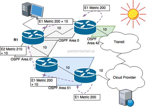
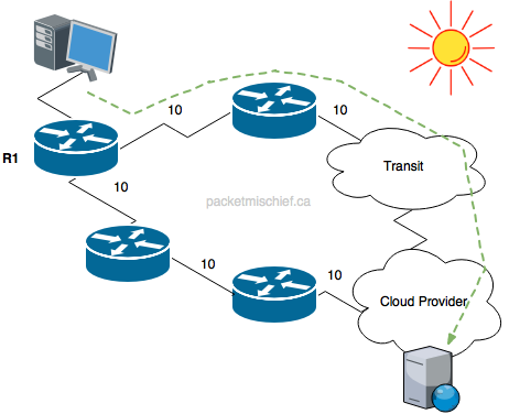
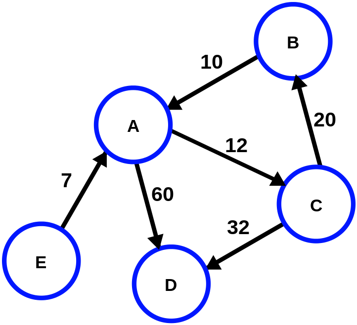
This might all be a little confusing, but don't dig too deeply into it. The important part is to realize that the type 1 metric (in E1/N1 routes) includes the external and internal metric to the off-net destination. You should be able to see now how the type 1 metric facilitates hot potato routing. Imagine an OSPF router (R1 in the diagram to the left) receives an E1 LSA from two different neighbors. The route via the first neighbor (top router, connected to transit) is quite attractive because that neighbor is very close to a network exit point. Also imagine the other path is far away from the interconnect and has a large metric to reach the interconnect. As long as the external part of the type 1 metric is the same or similar in the two LSAs, the OSPF router in question will prefer the E1 route being advertised by the first neighbor because it's closest to the exit. Hot potato!
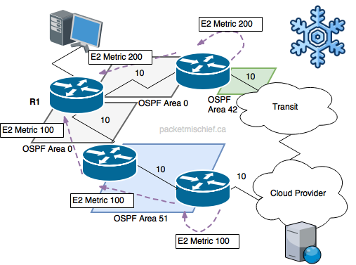
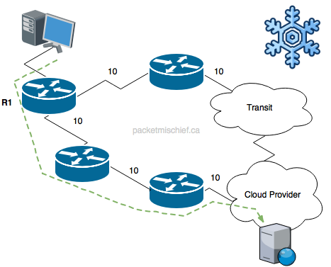
By contrast, cold potato routing uses the E2/N2 type LSAs which, you guessed it, use type 2 metrics. Type 2 metrics include only the external cost. This removes the on-net cost/metric from consideration and instead focuses on how close the ASBR is to the final destination. Again, imagine an OSPF router (R1) that receives an E2 LSA from two different neighbors. The LSA from the first neighbor (top router, connected to transit) advertises a high metric because it is relatively far away from the destination. The LSA from the second neighbor advertises a small metric because the OSPF border router (the ASBR) is relatively close to the source. R1 can now choose its path based on knowledge that the route via the second neighbor will get traffic to a border router that is much closer to the destination because the type 2 metric told it so.
Now, there is a big point of confusion with E2/N2 routes. While it's true that the metric itself is only the external cost, the internal cost is also carried in the LSA. In E1/N1, the internal and external costs are added together and carried as one composite number. In E2/N2, the internal cost is carried in a separate field of the LSA called the forward metric.
show ip route 192.168.0.0
Routing entry for 192.168.0.0/24
  Known via "ospf 1", distance 110, metric 20, type extern 2, forward metric 30
  Last update from 123.1.0.21 on Ethernet0/1, 3d06h ago
  Routing Descriptor Blocks:
* 123.1.0.21, from 10.1.12.12, 3d06h ago, via Ethernet0/1
      Route metric is 20, traffic share count is 1
The forward metric is used in the case where the regular type 2 metric is the same between two routes; the forward metric is the tie breaker.
3. OSPF is Built on a Database⌗
OSPF belongs to a family of protocols known as link state protocol. Link state protocols build a map of the entire network which includes the routers and the links/shared subnets that interconnect them. This map is called a directed graph and it is built by running an algorithm over the information in the link state database. When OSPF neighbors exchange routing information, they're not actually directly exchanging routes like the way BGP or EIGRP does, they're exchanging Link State Updates (LSUs) in an effort to fully synchronize the information in their databases.
One of the fundamental tenants of a link state protocol is that every router must have the same copy of the database. Once the databases are all in sync, each router can run the Djikstra algorithm over the database and come up with the map and hence the routing table. If the databases were out of sync, it's possible that routers would generate their routing tables in such a way that it led to a routing loop or maybe to some subnets being unreachable.
If you read carefully, you'll note I mentioned two discreet steps:
- Sync the database using LSUs
- Populate the routing table (the RIB) by running Djikstra over the database
It's really important to understand that these are two discreet steps. Step #1 always happens. You can't stop it. You can't filter it. It's a fundamental part of the protocol and like I mentioned, would lead to bad things if it wasn't happening. In fact, this is the basis for another article I wrote about using OSPF vs EIGRP for DMVPN. Understanding that Step #1 cannot be avoided is key to understanding why link state protocols are not suitable for DMVPN networks.
Step #2 is different though; that's where the network admin can exert some control. It is possible to filter routes that OSPF is pushing into the RIB. The LSA will still exist in the link state database, but it can be prevented from populating a route in the RIB and being used for traffic forwarding.
4. Reconvergence is Just a Matter of Time(rs)⌗
OSPF and the Djikstra algorithm where developed at a time when router CPU and memory were precious. As a result, the implementation in IOS and NX-OS (which are the ones I'll say I'm most familiar with) feature a number of timers designed to prevent the OSPF process from cratering the device during prolonged periods of network instability. These timers do their job but at the cost of slowing down convergence.
Once again let's use our imaginations and this time imagine an OSPF router with an OSPF-enabled interface that just came up. The router now needs to generate an LSA and send it to its neighbors. The very first time the interface comes up, the router immediately generates the LSA and advertises it in an LSU packet. Now let's assume the interface is not all that healthy and it's flapping up and down repeatedly. Without some sort of control, this would cause OSPF to repeatedly advertise a new LSA as fast as the interface was transitioning. Instead, there is a built-in throttling mechanism which backs off how often the same LSA can be advertised.
The first time the LSA needs to be advertised it is advertised immediately and a timer is started on the router. If that same LSA needs to be advertised again while the timer is running, the router waits until the timer expires, sends the LSA, and starts the timer again at double its previous value. This creates an exponentially rising back-off time. If the LSA doesn't need to be advertised during a period when the timer is running, the timer is reset to its initial value the next time it is started.
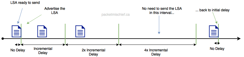
Basically what's happening is the first LSA goes out immediately but the software watches to see if that same LSA needs to be sent again within a short period of time. If that happens, the LSA is not sent (until the timer expires) and the timer is then doubled to increase the back-off time. The duration of the timer is capped at some maximum so it's not like hours or days can go by before that LSA can be advertised again. More like tens of seconds, at most.
The reason this affects convergence is in the case where the interface flaps just a couple of times and then remains stable. OSPF will go through a multi-second back-off all the same which will delay the rest of the network learning about the final state of that interface.
Another situation where OSPF uses throttling is when running the Shortest Path First (SPF) algorithm. Again, back to the theme of old routers having limited CPU: running SPF used to be very CPU intensive so preventing unnecessary runs of the algorithm helped keep routers happy. When a router receives an advertisement from a neighbor with some new topology information in it, it needs to run the Djikstra SPF algorithm against the databases in order to populate the RIB.
At a high level, SPF throttling will wait some amount of time the first time it learns of new topology information-just waiting to see if any additional information comes in-and then every subsequent time it will double the wait time, up to a defined maximum, creating an exponentially rising back-off time. If no new information is learned during a wait period, the wait time is reset to the initial wait value.
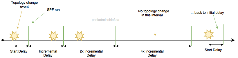
When it comes to Cisco IOS, the SPF throttle is a little more interesting than the LSA advertisement throttle because the SPF throttle kicks in the very first time SPF needs to run. That means there is an automatic delay before OSPF will run SPF which means there's a slightly longer period of time before the RIB and FIB are updated and traffic can begin flowing according to the new OSPF topology information. It's not uncommon to see these SPF throttling timers adjusted, but as always, be careful and if you don't fully grasp the impact of what you're changing, just leave it alone.
A far better way to avoid bumping up against OSPF's SFP throttling is to avoid needing to run SPF in the first place. If you can push network convergence from Layer 3 down to Layer 2 by employing more port channels in the network, you'll have a network that converges must faster.
5. The Link State Database is not a Routing Table⌗
I remember many years ago I had a router that was advertising an OSPF route (or at least I thought I did) to another router but I couldn't see the route installed in the RIB on the second router. I couldn't see any filters in the config that would be blocking the route from being installed in the RIB so I wanted to look in the OSPF database to see what OSPF was exchanging between the two routers.
This is about when my eyes started to cross.
What I didn't realize at the time is that the OSPF database describes the network topology, not the explicit L3 forwarding information. The L3 information is derived from the topology information at the time that SPF is run; in its native form in the database, the information is stored as LSAs, same as how they're advertised between neighbors. As a result, trying to glean whether a specific subnet (eg, 192.168.0.0/24) has been advertised between neighbors is more complicated than it would be when using a distance vector protocol such as EIGRP and RIP.
Let's look at an example.
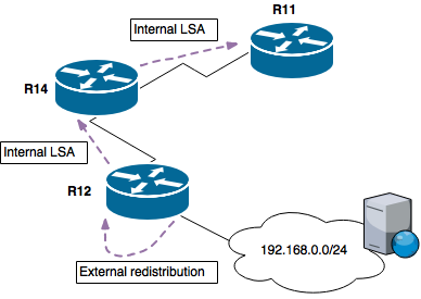
R12 is connected to 192.168.0.0/24 and is redistributing that network into OSPF (as a Type 5). That network is advertised through the OSPF domain and reaches R11 which is where we're going to inspect the OSPF database.
First we look in the OSPF database with show ip ospf database:
R11#show ip ospf database

            OSPF Router with ID (10.1.11.11) (Process ID 1)

                Router Link States (Area 0)

Link ID         ADV Router      Age         Seq#       Checksum Link count
10.1.11.11      10.1.11.11      1352        0x80000134 0x003ADD 3
10.1.12.12      10.1.12.12      100         0x800000BD 0x00B6F2 3
10.1.14.14      10.1.14.14      15          0x80000134 0x002A9B 5

                Type-5 AS External Link States

Link ID         ADV Router      Age         Seq#       Checksum Tag
192.168.0.0     10.1.12.12      1108        0x800000B9 0x00C595 0
You should notice right away that the 192.168.0.0 network shows up as the Link State ID of the sole external (Type 5) LSA in the database. I chose this example to show that external networks are pretty easy to identify in the database since the Link State ID is always equal to the network address. This is the same for inter-area routes as well (Type 3, aka "summary" types in the database).
Now for something a little harder. Let's look for intra-area network 123.1.1.0. At first glance it appears to be missing from the database. It's actually there, it's just not displayed in the high level output of the show ip ospf database command. To find it, we have to know something about the network topology. In this case I have the topology diagram so I know that 123.1.1.0/24 is the network connected to the e0/1 interface of R12. With this information, we can inspect the intra-area LSA-the "router LSA" that R12 originated:
R11#show ip ospf database router 10.1.12.12

            OSPF Router with ID (10.1.11.11) (Process ID 1)

                Router Link States (Area 0)
[...]
    Link connected to: a Stub Network
     (Link ID) Network/subnet number: 123.1.1.0
     (Link Data) Network Mask: 255.255.255.0
      Number of MTID metrics: 0
       TOS 0 Metrics: 10
Note I actually ran this command on R11. How does that work? Remember, all OSPF routers within the same area have the same copy of the database. You can inspect the database from any router in the area!
In this output we can see that 123.1.1.0 is a /24 network that's directly connected to R12 and is described as a "stub network" meaning there are no other OSPF speakers on that interface.
While this is slightly harder than looking at the external network, it still demonstrates how the OSPF database is built to reflect the network topology when it comes to intra-area networks. Additional examples could go on to show how sometimes multiple lookups need to be done to fully reverse engineer the topology by looking at the database but this article is already long so I will leave this out.
Disclaimer: The opinions and information expressed in this blog article are my own and not necessarily those of Cisco Systems.